Two Workloads in a Trench Coat: Why Prefill and Decode Change Everything

Part 1 of a 5-part series on LLM inference infrastructure.

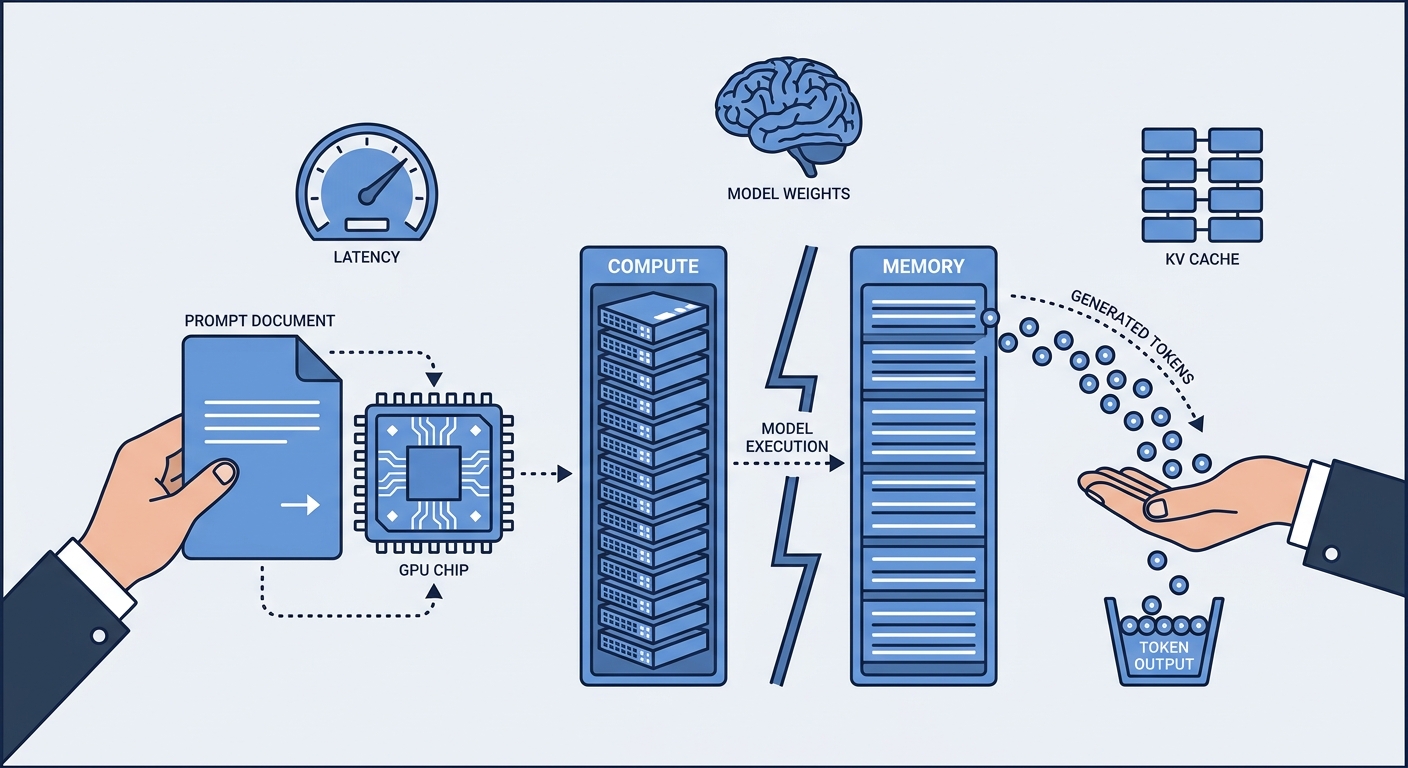
If you’ve spent your career building backend systems, you already have most of the mental furniture you need to understand how large language models are served. You know about load balancing, caching, memory hierarchies, head-of-line blocking, and virtual memory. What you probably don’t have yet is the one strange fact that makes LLM serving different from every other workload you’ve operated: a single inference request is secretly two completely different workloads wearing one trench coat. One half wants to saturate your GPU’s math units. The other half barely touches them and instead hammers memory bandwidth. They have opposite bottlenecks, opposite hardware preferences, and they actively sabotage each other when you run them together.

This series is my attempt to rewrite an earlier, denser post I wrote that a lot of people told me was too hard to follow. So I’m splitting it into five parts and slowing way down. In this first part, we’re going to build up — from absolute first principles — why the prefill/decode split exists, and then follow the historical thread of how the industry learned to deal with it: continuous batching, PagedAttention, and finally full prefill/decode disaggregation. By the end you’ll understand the architecture of systems like vLLM, NVIDIA Dynamo, and Mooncake well enough to reason about them. Let’s go.

What actually happens when an LLM answers you

Let’s start with tokens. An LLM doesn’t read characters or words; it reads tokens — chunks of text that have been mapped to integer IDs by a tokenizer. As a rule of thumb (OpenAI’s own Help Center gives these for English): 1 token ≈ 4 characters, 1 token ≈ ¾ of a word, and 100 tokens ≈ 75 words. The string "What is the capital of California: " might become a sequence of, say, eight token IDs. The model’s entire job is embarrassingly simple to state: given a sequence of tokens, predict the next one.

That’s it. The model is a next-token-prediction machine. To generate a full answer, you run it in a loop. You feed in the prompt, it predicts one token, you append that token to the sequence, you feed the whole thing back in, it predicts the next token, and so on until it emits a special end-of-sequence token or hits a length limit. This loop is called autoregressive generation — “autoregressive” just means each output depends on all the outputs before it. To borrow Anyscale’s example: prompt the model with “What is the capital of California: ” and it takes ten loop iterations to emit ["S","a","c","r","a","m","e","n","t","o"], one token per iteration.

Each pass of the model over its inputs is called a forward pass. Here’s the first thing that should bother you as a systems person: generating a 500-token answer means 500 forward passes through a model that might be tens or hundreds of gigabytes in size. That’s the seed of everything that follows.

Now, the key insight. These forward passes are not all alike. The very first one — where the model ingests your entire prompt — is fundamentally different from the 499 that follow.

Prefill: chewing the whole prompt at once

When your prompt arrives, the model processes all of its tokens in a single parallel forward pass. This is called prefill (or the “context” phase). Because every prompt token is already known up front, the GPU can process them all simultaneously — it’s a big, dense matrix-matrix multiplication, exactly the kind of work GPUs were built for. Prefill is compute-bound: it saturates the GPU’s floating-point math units (its FLOPs). If your prompt is 2,000 tokens long, prefill does roughly 2,000 tokens’ worth of work in one shot and keeps the tensor cores busy.

Decode: generating one token at a time

After prefill produces the first output token, you enter the decode (or “generation”) phase. Now you’re back in that autoregressive loop, and here’s the painful part: each forward pass generates exactly one token. You cannot parallelize across future tokens, because you don’t know token N+1 until you’ve computed token N. So decode is a long sequence of tiny forward passes, each one processing a single token.

This single-token-at-a-time structure is what makes decode memory-bandwidth-bound, and it’s worth understanding exactly why.

The KV cache: why we cache, and what it costs

To explain decode’s bottleneck I need to introduce the KV cache, which is the most important data structure in LLM serving.

Inside a transformer, the “attention” mechanism works by having each token look at every previous token. For each token, the model computes three vectors: a Query, a Key, and a Value (Q, K, V). To generate the next token, the model takes the current token’s Query and compares it against the Keys of all previous tokens, then uses those scores to take a weighted sum of their Values.

Here’s the problem: if you recomputed the Keys and Values for every previous token on every single decode step, your work would grow quadratically with sequence length — you’d redo all of history at every step. So instead we cache the Key and Value vectors for every token we’ve already processed. That cache is the KV cache. It’s a classic compute-for-memory trade, exactly like memoization in any backend system: spend RAM to avoid redoing work. With the KV cache, each decode step only needs to compute Q, K, V for the one new token, then read the cached K and V for all the old ones. Attention cost per step drops from quadratic to linear.

But now look at what every decode step has to do: it must read the entire model’s weights out of GPU memory (HBM, high-bandwidth memory) plus the entire KV cache, just to produce one token. The weights might be 140 GB for a 70-billion-parameter model in 16-bit precision. You’re moving all of that across the memory bus to do a comparatively tiny amount of math on a single token. That’s the definition of memory-bandwidth-bound.

How big is the KV cache, concretely?

Let’s compute it, because the number surprises people. The standard formula for the KV cache size per token is:

bytes per token = 2 × num_layers × hidden_size × bytes_per_value

The leading 2 is for storing both Keys and Values. Take Llama 2 7B in FP16 (2 bytes/value): it has 32 layers and a hidden size of 4096. So per token:

2 × 32 × 4096 × 2 = 524,288 bytes ≈ 512 KB per token

For a full 4,096-token context, that’s 512 KB × 4096 ≈ 2 GB of KV cache — for a single request. NVIDIA’s own inference-optimization guide works exactly this example and lands at ~2 GB. Now imagine batching 10 requests: that’s 20 GB of KV cache on top of your 14 GB of model weights, and you start to see why memory, not compute, is the thing that runs out first.

Arithmetic intensity and the roofline: putting numbers on the bottleneck

Systems engineers love a good back-of-the-envelope model, so here’s the one that governs everything in LLM inference: the roofline model.

Define arithmetic intensity as the number of floating-point operations you perform per byte you move from memory (FLOPs/byte). Every GPU has a break-even point — call it the ridge point — where its peak compute exactly balances its peak memory bandwidth. Below that intensity, you’re memory-bound (starved for data); above it, you’re compute-bound (starved for math units).

Let’s compute the ridge point for an NVIDIA H100 SXM. Its datasheet specs are precise: 989 FP16/BF16 TFLOPS (dense) — the figure doubles to 1,979 TFLOPS only with structured sparsity — and 3,350 GB/s of HBM3 memory bandwidth, across 80 GB of HBM3. The ridge point is:

989 × 10¹² FLOPs/s ÷ 3.35 × 10¹² bytes/s ≈ 295 FLOPs/byte

So to keep an H100 busy, you need to do ~295 floating-point operations for every byte you pull from memory. Now, what’s the arithmetic intensity of decode? Single-token decode is essentially a matrix-vector product: you read a big weight matrix (many bytes) and multiply it by a single token’s activation vector (very little math). Its arithmetic intensity is roughly 1 FLOP/byte. The ridge point is ~295. The gap is two orders of magnitude. This is not an inefficiency you can tune away — it’s structural. During decode, the most expensive compute silicon on Earth sits idle the overwhelming majority of the time, waiting for memory.

We can even compute the speed ceiling. A 70B model in FP16 is ~140 GB of weights. On an H100’s 3.35 TB/s bus, reading all the weights once takes 140 / 3350 ≈ 42 ms. Since each decode token requires reading all the weights, your single-user decode ceiling is about 3350 / 140 ≈ 24 tokens per second, no matter how fast the math units are. Prefill, by contrast, processes thousands of tokens in parallel, so it easily clears the 295 ridge point and becomes compute-bound.

This is the whole ballgame. Prefill is compute-bound; decode is memory-bandwidth-bound. One workload, two personalities. The analogy I like: prefill is a batch ETL job that pegs your CPUs; decode is a chatty, latency-sensitive request handler that mostly waits on I/O. You would never run those two on identically tuned infrastructure if you had the choice — and the rest of this post is the story of the industry slowly realizing exactly that.

There are two latency metrics you’ll see everywhere, and they map cleanly onto the two phases. TTFT (time to first token) is dominated by prefill — how long until the user sees anything. TPOT (time per output token, also called inter-token latency) is dominated by decode — how fast the words stream out after that. A chatbot wants low TTFT and a TPOT that comfortably beats human reading speed; a code-completion tool wants blistering end-to-end speed. Different apps weight these differently, which matters enormously later.

Why naive batching wastes your GPUs

Since decode is memory-bound and barely uses the compute, the obvious fix is batching: process many requests at once so that when you read the model weights from memory, you amortize that read across many sequences. Load the weights once, do the math for 32 requests. Batching is how you claw back GPU utilization, and it’s the single most important throughput lever in LLM serving.

The naive way to do this is static batching (also called request-level batching): collect N requests, run them all together until every one of them finishes, then start the next batch. If you’ve ever operated an HTTP server, you’ll smell the problem instantly — it’s head-of-line blocking.

Here’s the failure in detail. Suppose you batch 8 requests. Seven of them generate 30-token answers and finish quickly. One generates 400 tokens. With static batching, those seven finished sequences just sit there, occupying slots in the batch, doing padding work, while the GPU grinds through the one long straggler. Anyscale measured exactly this on OPT-13B: as the variance in output lengths grows, static-batching throughput collapses. The GPU is underutilized for the entire tail of the batch — and in a real chatbot, where output lengths are wildly unpredictable, that tail is most of the time.

Orca: scheduling at the granularity of a single iteration

The fix came from a 2022 OSDI paper, Orca: A Distributed Serving System for Transformer-Based Generative Models (Yu et al., from Seoul National University and FriendliAI). Orca introduced two ideas that together define modern serving.

The first is iteration-level scheduling (this is what everyone now calls continuous batching). Instead of the scheduler picking a batch and waiting for it to finish, the scheduler runs once per decoding iteration. After every single token-generation step, it can retire requests that just finished and admit brand-new requests into the empty slots — mid-flight, without waiting for the rest of the batch. The batch composition changes every iteration. The instant a sequence emits its end-of-sequence token, its slot is freed and a waiting request jumps in. No more head-of-line blocking; the GPU stays full.

The second idea solves a subtle implementation snag. Once you allow requests at different stages to share a batch, you have a shape problem: a request doing prefill has many tokens; a request doing decode has one; their cached Keys and Values have different lengths. You can’t just stack them into one neat tensor. Orca’s answer is selective batching: batch the operations that don’t care about per-request boundaries (the big Linear, LayerNorm, and activation layers, which just see a flat pile of tokens) and handle the attention operation separately per-request (since attention is the one operation that needs each sequence’s own history). The paper found that not batching attention has only a small efficiency cost — a fantastic trade.

The results were dramatic. On a GPT-3 175B model, Orca reported a 36.9× throughput improvement over NVIDIA FasterTransformer at the same latency level. Concretely, to hold a 190 ms latency target, FasterTransformer managed 0.185 requests/second while Orca delivered 6.81 — that’s the 36.9×.

Anyscale later reproduced the idea on more modest hardware (OPT-13B on a single A100 40 GB) and published widely-cited numbers: continuous batching delivered up to 23× throughput over naive HuggingFace Transformers (when combined with vLLM’s memory optimizations), and about 8× from continuous batching alone over naive batching. Today continuous batching is table stakes — it’s the default in vLLM, HuggingFace TGI (text-generation-inference), and TensorRT-LLM. If you deploy any modern serving stack, you’re using Orca’s ideas whether you know it or not.

PagedAttention: virtual memory for the KV cache

Continuous batching fixed when we schedule requests. But it exposed a second, deeper problem: where do we put all those KV caches? This is where vLLM and PagedAttention enter, from the 2023 SOSP paper “Efficient Memory Management for Large Language Model Serving with PagedAttention” by Kwon et al. at UC Berkeley.

Here’s the pre-vLLM situation. A request’s KV cache grows token by token, but you don’t know in advance how long the output will be. So the simplest thing systems did was pre-allocate one big contiguous block of GPU memory per request, sized to the maximum possible sequence length. If your model supports 2,048 tokens, every request reserved room for 2,048 tokens’ worth of KV cache up front — even if it ultimately generated 20.

If you’ve ever managed a memory allocator, you know what happens next. You get internal fragmentation (the reserved-but-never-used tail of each request’s block), reservation waste (memory reserved for future tokens that hasn’t been generated yet), and external fragmentation (leftover gaps between blocks too small to use). The vLLM paper measured that existing systems were actually using only 20–38% of the memory they allocated for KV cache — meaning 60–80% was wasted. And since KV cache capacity is what caps your batch size, wasting it directly throttles throughput.

The fix is one of those ideas that’s obvious in hindsight to anyone who’s studied an operating system: stop demanding contiguous memory. PagedAttention borrows OS virtual memory and paging wholesale. It chops the KV cache into fixed-size blocks of 16 tokens each. These blocks can live anywhere in GPU memory — non-contiguously. Each sequence gets a block table that maps its logical block numbers (logical block 0, 1, 2…) to wherever the physical blocks actually sit. That block table is precisely an OS page table; the 16-token blocks are pages; the indirection is identical. Blocks are allocated on demand as a sequence grows, and returned to a free pool when it finishes.

The payoff: memory waste drops from 60–80% to under 4% (the only waste is the last partially-filled block per sequence). With that reclaimed memory you can fit far bigger batches, and bigger batches mean higher throughput on a memory-bound workload. The original vLLM paper reported up to 24× higher throughput than HuggingFace Transformers and up to 3.5× over HuggingFace TGI, and 2–4× over FasterTransformer and Orca at the same latency. The real-world proof point: LMSYS, who run Chatbot Arena, cut their GPU count by 50% while serving 2–3× more traffic after adopting vLLM.

Sharing blocks: prefix caching and copy-on-write

Paging unlocks a bonus trick. If multiple requests share the same prefix — say, an identical 500-token system prompt that every user request begins with — why store and compute it more than once? Because KV cache is now just blocks behind a block table, multiple sequences can simply point their block tables at the same physical blocks. This is prefix caching, and it uses copy-on-write exactly like fork() in an OS: the shared prefix blocks stay shared and read-only; the moment a sequence needs to write a token that diverges, just that one block is copied. The vLLM paper showed this cuts memory by up to 55% for beam search and yields large savings whenever prefixes are shared.

SGLang generalized this beautifully with RadixAttention (Zheng et al., arXiv:2312.07104, from LMSYS; published at NeurIPS ‘24). Instead of caching just one shared prefix, it stores all cached prefixes in a radix tree — a space-efficient prefix tree — keyed by token sequences, with an LRU eviction policy. When a new request arrives, SGLang walks the tree to find the longest matching prefix already in cache and reuses its KV blocks, computing only the new suffix. Picture a chatbot where thousands of requests share a system prompt, then branch into different conversations, then branch again per turn — that’s a tree, and RadixAttention caches every internal node. The paper reports cache hit rates ranging from 50% to nearly 99% across benchmarks and achieves up to 6.4× higher throughput versus state-of-the-art systems (and reduces latency by up to 3.7× on Llama-7B). The catch worth knowing: the prefix must match byte-for-byte in token IDs, so a single changed character upstream invalidates the cache for everything downstream.

Prefill/decode disaggregation: stop making them fight

Now we arrive at the frontier, and it brings us full circle to the trench-coat metaphor.

Even with continuous batching and PagedAttention, by default you run prefill and decode on the same GPU, interleaved by the scheduler. Remember they have opposite personalities. So watch what happens: a long prefill (compute-bound, hogs the math units for many milliseconds) lands in the batch, and every latency-sensitive decode step for other users gets stalled behind it. The decode requests — which just wanted their next token quickly — see their TPOT spike. This is prefill-decode interference. It’s head-of-line blocking again, but now between two workloads with fundamentally different SLAs sharing one device.

The DistServe paper (Zhong et al., OSDI 2024, from Peking University and UCSD’s Hao AI Lab) made the case for the clean fix: put prefill and decode on separate pools of GPUs. Prefill GPUs do nothing but chew prompts; decode GPUs do nothing but stream tokens. After a prefill GPU finishes computing a request’s KV cache, it ships that cache over the network to a decode GPU, which takes over generation.

This buys two things. First, no more interference — a long prefill can’t stall anyone’s decode, because they’re on different machines. Second, independent scaling and tuning: the two phases can use different degrees of parallelism, different batch sizes, even different GPU types, each tuned for its own bottleneck.

DistServe also reframed the success metric. Raw throughput (tokens/second) is the wrong target if half those tokens blew their latency budget. The right metric is goodput: the number of requests completed per second that actually meet their TTFT and TPOT SLOs. Optimizing goodput is what aligns the system with user experience and cost. DistServe reported it could serve 7.4× more requests or meet 12.6× tighter SLOs than then-current systems while staying within latency constraints for over 90% of requests; against vLLM specifically it sustained 2.0×–4.6× higher request rate on the ShareGPT chatbot workload, and its blog reported 4.48× higher goodput than vLLM on a summarization workload.

How the KV cache actually moves: NIXL

Disaggregation only works if you can move the KV cache from a prefill GPU to a decode GPU fast, because that transfer sits on the critical path to first token. Shipping gigabytes through CPU memory and a TCP socket would obliterate your TTFT. The answer is NIXL (NVIDIA Inference Transfer Library), open-sourced by NVIDIA at GTC 2025. NIXL is a point-to-point data-transfer library that does GPU-to-GPU transfers directly, without a CPU round-trip, and non-blocking, so the GPUs can keep running forward passes for other requests while the KV cache moves in the background. Crucially, it’s an abstraction layer over many transports — it automatically picks the best available path among RDMA/InfiniBand, RoCE (via UCX), plain TCP, NVLink, NVMe-oF, and even S3-compatible object storage — so your serving code doesn’t have to care whether two workers are NVLinked in the same box or sitting across an InfiniBand fabric.

NVIDIA Dynamo: the orchestration layer

NVIDIA Dynamo is the open-source, datacenter-scale framework that productionizes all of this. It’s not a replacement for vLLM, SGLang, or TensorRT-LLM — it sits above them and coordinates a fleet of them. Its key pieces map neatly onto concepts you already know:

• A KV-aware (smart) router routes each request to the worker most likely to already have its prefix cached, minimizing redundant prefill — like a cache-affinity load balancer.
• A global prefill queue, implemented on NATS (a high-performance messaging system), where prefill work is posted and prefill workers pull from it — a classic work queue decoupling producers from consumers.
• etcd for service discovery: workers register their endpoints and their NIXL memory descriptors (so peers know where to write KV blocks), and the router discovers them — the same etcd you’ve probably used for Kubernetes coordination.
• A GPU Planner that autoscales the prefill and decode pools independently, watching the prefill-queue depth to size the prefill pool and average KV-cache utilization to size the decode pool.

NVIDIA published a headline figure of up to 30× more requests serving DeepSeek-R1 671B on GB200 NVL72 racks with disaggregated serving versus an inflight-batching baseline — but be careful with this one: NVIDIA explicitly labels it “projected performance subject to change,” not a measured production result, and it applies to a specific TensorRT-LLM FP4 / 32K-input configuration. A more recent, independently benchmarked figure (attributed to SemiAnalysis InferenceX) is up to 7× MoE throughput for DeepSeek-R1 on GB200 NVL72 versus B200-based systems — again a combined hardware-plus-software comparison, not pure disaggregation. Don’t merge the two numbers; they use different baselines, models, and sequence lengths.

The wider ecosystem: Mooncake and llm-d

Dynamo isn’t alone. Mooncake is the KVCache-centric disaggregated platform that serves Kimi, Moonshot AI’s production LLM. It separates prefill and decode clusters and pools the otherwise-idle CPU, DRAM, and SSD across the GPU fleet into a giant disaggregated KV-cache tier. In the peer-reviewed USENIX FAST ‘25 version of their paper, the team reports that in production, Mooncake’s architecture let Kimi handle 115% and 107% more requests on NVIDIA A800 and H800 clusters respectively versus their previous systems (the higher “525% throughput” number you’ll see quoted is from simulated scenarios in the preprint, so treat it accordingly), and that the system runs across thousands of nodes processing over 100 billion tokens daily.

llm-d is the Kubernetes-native take, launched by Red Hat, Google, IBM Research, CoreWeave, and NVIDIA, and accepted into the CNCF Sandbox. It builds on vLLM and standard Kubernetes primitives (the Gateway API Inference Extension, CRDs) rather than a separate control plane, and offers prefill/decode disaggregation, cache-aware routing, and tiered KV offloading as composable “well-lit paths.” Where Dynamo is an orchestration layer outside Kubernetes tuned for NVIDIA’s stack, llm-d is a first-class Kubernetes citizen — pick based on where your platform team already lives.

The economics, honestly

You’ll see a widely-repeated claim that disaggregation cuts cost-per-token by roughly 3–5× on chat workloads. I dug for a clean primary source on that exact “3–5×” figure and couldn’t find one — it appears to be a secondhand synthesis, so I’d treat it as a rule-of-thumb rather than a measured fact. What I can point to with primary backing is the underlying mechanism: DistServe’s 7.4× more requests per GPU at fixed SLOs and Mooncake’s production ~110% more requests, both of which translate directly into fewer GPUs per unit of served traffic, i.e. lower cost per token. The other big lever is hardware heterogeneity: because decode is memory-bound and prefill is compute-bound, you can put cheaper or older GPUs on one phase and reserve premium silicon for the other, which a colocated design can never do.

Life of a single request, end to end

Let’s tie it together by following one request through a disaggregated Dynamo-style system, step by step:

1. Arrival. Your HTTP request hits the frontend (an OpenAI-compatible API server).
2. Routing. The KV-aware router checks which prefill worker is most likely to already hold your prompt’s prefix in cache, balancing that against current load, and picks one.
3. Enqueue. The request — carrying the IDs of pre-allocated KV blocks on the destination decode worker — is pushed onto the global prefill queue on NATS.
4. Prefill. A prefill worker pulls the job, runs the big compute-bound parallel forward pass over your whole prompt, and produces the KV cache (and the first token).
5. Transfer. Using NIXL, the prefill worker writes the KV blocks directly into the decode worker’s GPU memory over the best available transport (NVLink, InfiniBand, etc.), non-blocking, with no CPU in the middle. The prefill GPU is immediately free to grab the next job from the queue.
6. Decode. The decode worker, which has been continuously batching other users’ generations the whole time, slots your request in and begins the memory-bound autoregressive loop, streaming one token per iteration back to you.
7. Completion. When your sequence emits its end-of-sequence token, the decode worker frees your KV blocks back to the pool (PagedAttention), and continuous batching admits the next waiting request into your slot.

Every concept in this post shows up in that one request: prefill vs. decode, the KV cache, paging, continuous batching, KV-aware routing, and disaggregated transfer.

Recap

Here’s the whole arc in one breath. An LLM answers by predicting one token at a time in an autoregressive loop, and that loop splits into two opposite workloads: prefill processes your whole prompt in one parallel, compute-bound pass, while decode generates tokens one at a time and is memory-bandwidth-bound because every token requires re-reading all the model weights and the KV cache from HBM. We quantified this with the roofline model: an H100’s ridge point is ~295 FLOPs/byte, but decode runs at ~1, so the compute units sit mostly idle. The KV cache exists to avoid recomputing attention history, but it’s huge (≈2 GB for one 4K-token Llama-2-7B request) and its management is the central engineering problem.

The industry solved this in three waves. Continuous batching (Orca, 2022) reschedules every iteration to kill head-of-line blocking, for up to 36.9× gains. PagedAttention (vLLM, 2023) applies OS-style paging to slash KV-cache waste from 60–80% down to under 4%, enabling up to 24× throughput, plus prefix sharing via copy-on-write (and SGLang’s RadixAttention generalization, up to 6.4×). And prefill/decode disaggregation (DistServe, 2024) puts the two workloads on separate, independently-scaled GPU pools to eliminate interference and optimize goodput (7.4× more requests) — now productionized in NVIDIA Dynamo, Mooncake, and llm-d, with NIXL doing the fast GPU-to-GPU KV transfer underneath.

Coming up in Part 2

We’ve been talking about architecture — but who’s paying? In Part 2, we’ll follow the money: how MoE, quantization, and caching stack multiplicatively to produce a 545% theoretical profit margin, why inference costs collapsed 280× in two years, and the 40% utilization threshold that decides whether you should self-host or buy API tokens.